Flyers 4 - Flyers v3: Azure Data Factory

project flyers

Flyers v3: Azure Data Factory

Introduction
Version 1
Version 2
Version 3
Reporting Dashboard
Data Cleansing
Power BI Results
~~MS Fabric (v4)~~
~~AI with Power BI~~

This is part four of a series of short blogs chronicling a pet project I’ve come to know as Flyers. Flyers is a data exploration journey to capture authentic sale prices from local grocery stores and use that data to visualize trends over time. ~~Files associated with this project are available at https://github.com/carsonruebel/Flyers~~. This article covers the third solution I arrived at, which utilizes Azure Data Factory (ADF) to extract, transform, and load data from an API to an Azure SQL DB on a daily basis.

This version, developed with Azure Data Factory, represents the final rendition accomplished during the original creation of this project in early 2022. Following the completion of this version, I transitioned to a new role and deemed it sufficiently stable to continue executing and gather data over an extended period.

Azure Data Factory

In Microsoft’s own words, Azure Data Factory is Azure’s serverless extract, transform, and load (ETL) solution. It offers a simple graphical user interface that is used to piece together the process of extracting, transforming, and loading data from a source to a sink. This was my first project using ADF, and although I found it simple enough to set up, I now realize there were steps I should have done differently. In this rebuild, I clean up some of those inefficiencies.

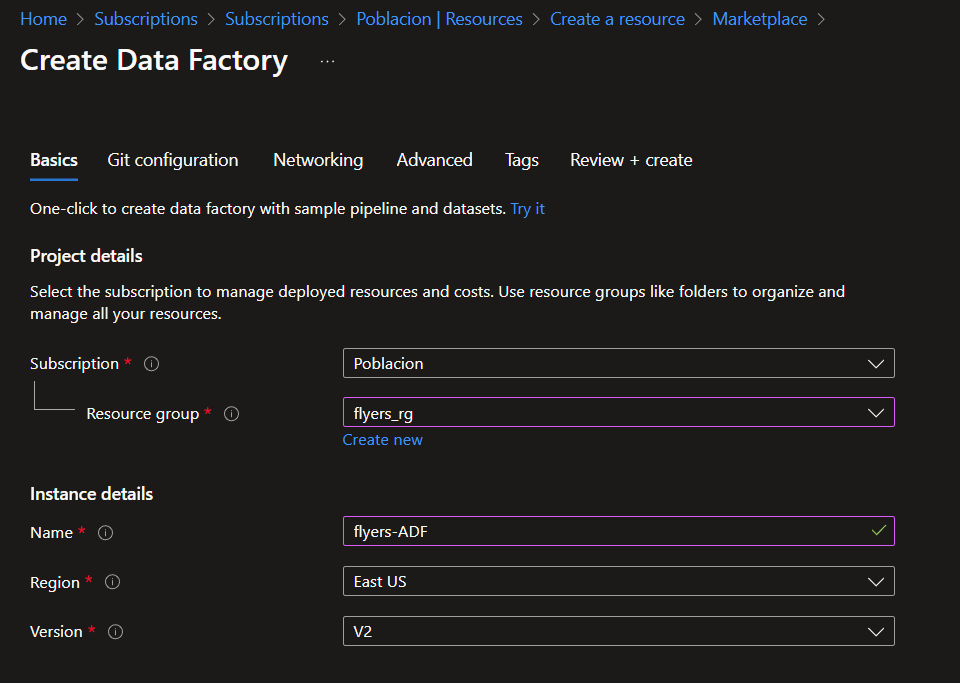
The first step in setting up ADF is to create a Data Factory resource within your subscription. For my solution, I will use the name ‘flyers-ADF’.

Now that we have the Data Factory set up, we need to start configuring it. Within the resource, you will be able to launch the Azure Data Factory Studio, which is where all the configurations will occur. Under the ‘Author’ tab within Azure Data Factory, there are three main resources we will need to make use of.

Pipelines: Pipelines are used for process orchestration; organizing and connecting individual activities within Azure Data Factory. Pipelines are made up of activities. We will encapsulate the entire ETL within one pipeline activity as all of the work relates to data transformation.
Datasets: Datasets represent either a source or a destination (sink). We will need one dataset for each store we are pulling data from, and one for our SQL DB as a sink. A dataset is merely a named pointer for a dataset. In order to connect to that dataset, we will need to create a connection string via a linked service. Linked services are used to connect resources to Azure Data Factory.
Dataflows: Dataflows are used for data transformation and are made up of transformations. This is where the bulk of our work will occur.

Create Datasets

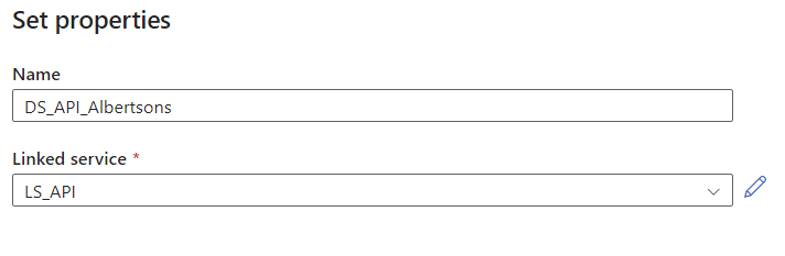
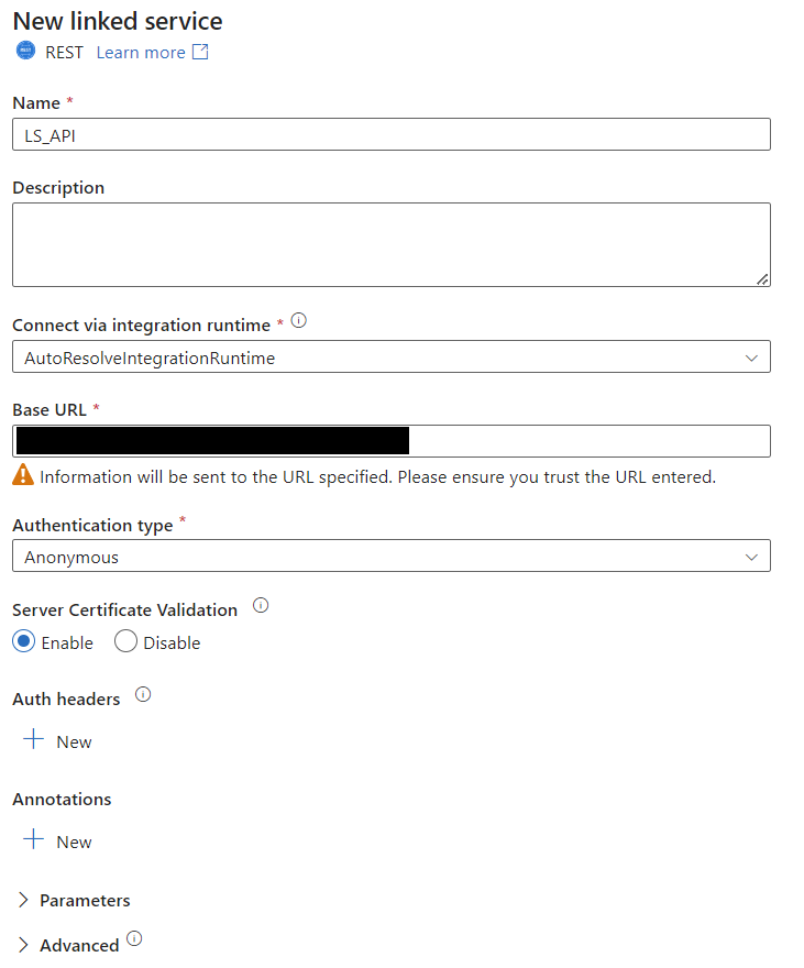
Let’s begin by creating a dataset to represent one of the stores. We will be pulling data from a RESTful API, so select ‘New Dataset’ under the dataset section and search for REST. The creation screen will ask for a name and a linked service. Select ‘New’ under the linked service dropdown to bring up the creation prompt for linked services. We will be utilizing the same API for each store, just feeding it a different parameter for each. Therefore, we will be able to use the same linked service REST connection for all the stores. Set the Base URL of the linked service to ‘████████’ and set the authentication type to anonymous.

You can now see your first dataset in the ‘Author’ tab under datasets. You can also test the connection with the built-in ‘Test connection’ button.

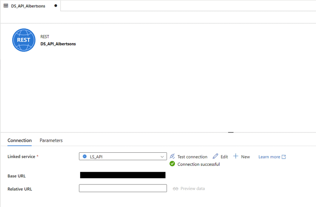
In order to have this dataset point to a specific store, we will need to tell Azure Data Factory some additional information to use in the API. I know of at least three parameters that can be used with this API: locale, postal_code, and q. We will use these three to specify language, geographic location, and store name. In the ‘Relative URL’ field, enter the following, then publish the changes.

?locale=en-us&postal_code=98125&q=Albertsons

That’s all there is to setting up data sources that pull from an API. You can go through the same steps to create new datasets that connect to the linked service for the remaining stores, or you can click the dropdown menu from the first dataset and select ‘Clone’ to build out and configure the Relative URL for the remainder of stores. For this project, that means creating four additional datasets using the following Relative URLs. Don’t forget to publish your changes after creating them.

?locale=en-us&postal_code=98125&q=FredMeyer
?locale=en-us&postal_code=98125&q=QFC
?locale=en-us&postal_code=98125&q=Safeway
?locale=en-us&postal_code=98125&q=Walmart

We have now configured the sources, but we still need to specify a destination. We will be storing the results of the API pulls in our Azure SQL DB. To do this, we’ll need to create a new dataset and linked service to connect to our database. Before doing this, let’s preemptively grant permissions for ADF to manage our DB. In SSMS, run the following two commands within the context of the flyersdb database. This will create a SQL user for the ADF resource and grant it full ownership permission. Note that this uses the name of our ADF resource. In this case it is ‘flyers-ADF’.

CREATE USER [flyers-ADF] FROM EXTERNAL PROVIDER;
ALTER ROLE db_owner ADD MEMBER [flyers-ADF];

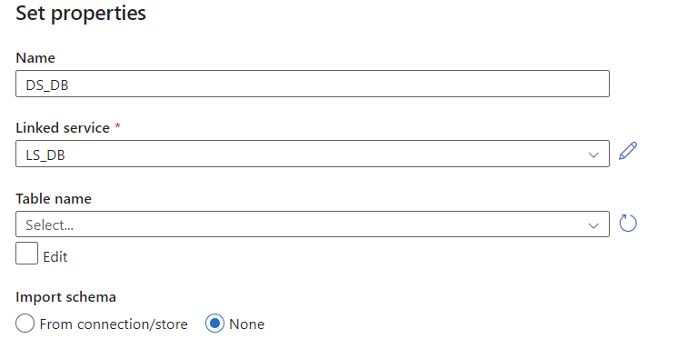
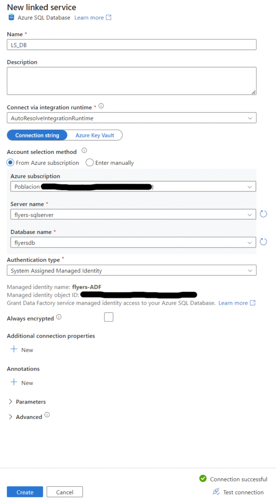
Now we can go ahead and create the dataset and linked service for our Azure SQL Database. For the linked service configuration, point it to the correct database that we created for this project and select ‘System Assigned Managed Identity’ as the authentication type. You could also do a basic username and password via SQL authentication if you set up your SQL server that way and prefer it. Before creating, test the connection in the bottom right. If we had not properly granted permissions in the database first, this test would fail. We will leave the table name blank for now and come back to set it up later.

Setup Sink (SQL DB)

Before we start working on the actual dataflow within ADF, it will be helpful if we set up the sink first. The sink refers to the destination for the data to go after transformation in ADF is complete. Similar to the v2 solution, we’ll create a v3 set of tables. We’ll also make use of a staging table within our SQL DB. This will mimic the input sheets we had in v1 and v2 which will need to be normalized to dim and fact tables. To create these tables, we’ll use the queries below.

CREATE TABLE Staging_v3 (
    AdID INT IDENTITY(1,1) PRIMARY KEY NOT NULL,
    Load_Date DATE NOT NULL,
    Industry VARCHAR(255) NULL,
    _L1 VARCHAR(255) NULL,
    _L2 VARCHAR(255) NULL,
    clean_image_url VARCHAR(255) NULL,
    clipping_image_url VARCHAR(255) NULL,
    current_price DECIMAL(10,2) NULL,
    flyer_id INT NULL,
    flyer_item_id INT NULL,
    id INT NULL,
    item_type VARCHAR(255) NULL,
    merchant_id VARCHAR(255) NULL,
    merchant_logo VARCHAR(255) NULL,
    merchant_name VARCHAR(255) NULL,
    name VARCHAR(255) NULL,
    original_price INT NULL,
    post_price_text VARCHAR(255) NULL,
    pre_price_text VARCHAR(255) NULL,
    sale_story VARCHAR(255) NULL,
    valid_from VARCHAR(255) NULL,
    valid_to VARCHAR(255) NULL
);

CREATE TABLE DIM_Industry_v3 (
    IndustryID INT IDENTITY(1,1) PRIMARY KEY NOT NULL,
    Industry VARCHAR(50) NOT NULL
);

CREATE TABLE DIM_Merchant_v3 (
    MerchantID INT IDENTITY(1,1) PRIMARY KEY NOT NULL,
    Merchant VARCHAR(100) NOT NULL
);

CREATE TABLE DIM_Product_v3 (
    ProductID INT IDENTITY(1,1) PRIMARY KEY NOT NULL,
    Brand_Product VARCHAR(100) NOT NULL,
    Category VARCHAR(100) NULL,
    pre_price_text VARCHAR(100) NULL,
    URI VARCHAR(255) NOT NULL
);

CREATE TABLE FACT_Ad_v3 (
    AdID INT IDENTITY(1,1) PRIMARY KEY NOT NULL,
    LoadDate DATE NOT NULL,
    StartDate DATE NOT NULL,
    EndDate DATE NOT NULL,
    IndustryID INT FOREIGN KEY REFERENCES DIM_Industry_v3(IndustryID) NOT NULL,
    MerchantID INT FOREIGN KEY REFERENCES DIM_Merchant_v3(MerchantID) NOT NULL,
    ProductID INT FOREIGN KEY REFERENCES DIM_Product_v3(ProductID) NOT NULL,
    Price DECIMAL(10,2) NOT NULL
);

Since we are using the same API source for the data, there are almost no changes to the dim and fact tables from v2. The only difference is that we add a ‘LoadDate’ attribute to the fact table. Since we will eventually have this pipeline run on a daily basis, it makes sense to create a load date attribute in case we ever need it for troubleshooting or analysis.

The attributes in the Staging table are all the attributes I ended up seeing as potentially valuable. Not every attribute is used in the dim/fact tables, but for this small volume of data, it doesn’t hurt to have them flow into the staging table in case I choose to start storing and using these attributes in the future.

Like we did in the first two versions, we need a stored procedure to transform the data from a human-readable format to dim and fact tables. This stored procedure is more complex than the first two as it uses a SQL table as a source instead of being executed separately for each row. This means we need to use a cursor to iterate through the records, which are then split into dim and fact tables as we have in the past. At the end, we clean up the staging table to reset it to an empty usable state for the next time the ADF pipeline runs. Note this query contains an error that caused data issues further down the line. The correction and impact is discussed in this post.

CREATE PROCEDURE InsertNormalizedAd_v3 AS
BEGIN
    DECLARE @industry VARCHAR(50)
    DECLARE @merchant VARCHAR(100)
    DECLARE @brandproduct VARCHAR(100)
    DECLARE @productcategory VARCHAR(100)
    DECLARE @prepricetext VARCHAR(100)
    DECLARE @uri VARCHAR(255)
    DECLARE @startdate DATE
    DECLARE @enddate DATE
    DECLARE @price DECIMAL(10,2)
    DECLARE @loaddate DATE

    DECLARE c CURSOR FOR
        SELECT Industry, merchant_name, name, _L2, pre_price_text, clean_image_url, valid_from, valid_to, current_price, Load_Date
        FROM Staging_v3
        WHERE current_price IS NOT NULL

    OPEN c
    FETCH NEXT FROM c INTO @industry, @merchant, @brandproduct, @productcategory, @prepricetext, @uri, @startdate, @enddate, @price, @loaddate

    WHILE @@FETCH_STATUS = 0
    BEGIN
        DECLARE @industryid INT;
        SET @industryid = (SELECT IndustryID FROM DIM_Industry_v3 WHERE Industry = @industry);
        IF @industryid IS NULL
        BEGIN
            INSERT INTO DIM_Industry_v3 VALUES (@industry);
            SET @industryid = (SELECT IndustryID FROM DIM_Industry_v3 WHERE Industry = @industry);
        END

        DECLARE @merchantid INT;
        SET @merchantid = (SELECT MerchantID FROM DIM_Merchant_v3 WHERE Merchant = @merchant);
        IF @merchantid IS NULL
        BEGIN
            INSERT INTO DIM_Merchant_v3 VALUES (@merchant);
            SET @merchantid = (SELECT MerchantID FROM DIM_Merchant_v3 WHERE Merchant = @merchant);
        END

        DECLARE @productid INT;
        SET @productid = (SELECT ProductID FROM DIM_Product_v3 WHERE Brand_Product = @brandproduct);
        IF @productid IS NULL
        BEGIN
            INSERT INTO DIM_Product_v3 VALUES (@brandproduct, @productcategory, @prepricetext, @uri);
            SET @productid = (SELECT ProductID FROM DIM_Product_v3 WHERE Brand_Product = @brandproduct);
        END

        INSERT INTO FACT_Ad_v3 VALUES (@loaddate, @startdate, @enddate, @industryid, @merchantid, @productid, @price);

        FETCH NEXT FROM c INTO @industry, @merchant, @brandproduct, @productcategory, @prepricetext, @uri, @startdate, @enddate, @price, @loaddate
    END;

    CLOSE c
    DEALLOCATE c

    DELETE FROM Staging_v3;
    DBCC CHECKIDENT ('Staging_v3', RESEED, 0);
END
GO

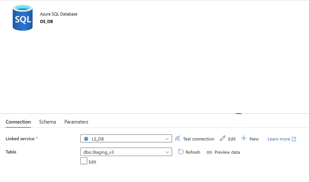
We can now go back into the DB dataset and point it to the staging table we created. You will likely need to hit the ‘Refresh’ button for the newly created tables to appear.

ADF Dataflow

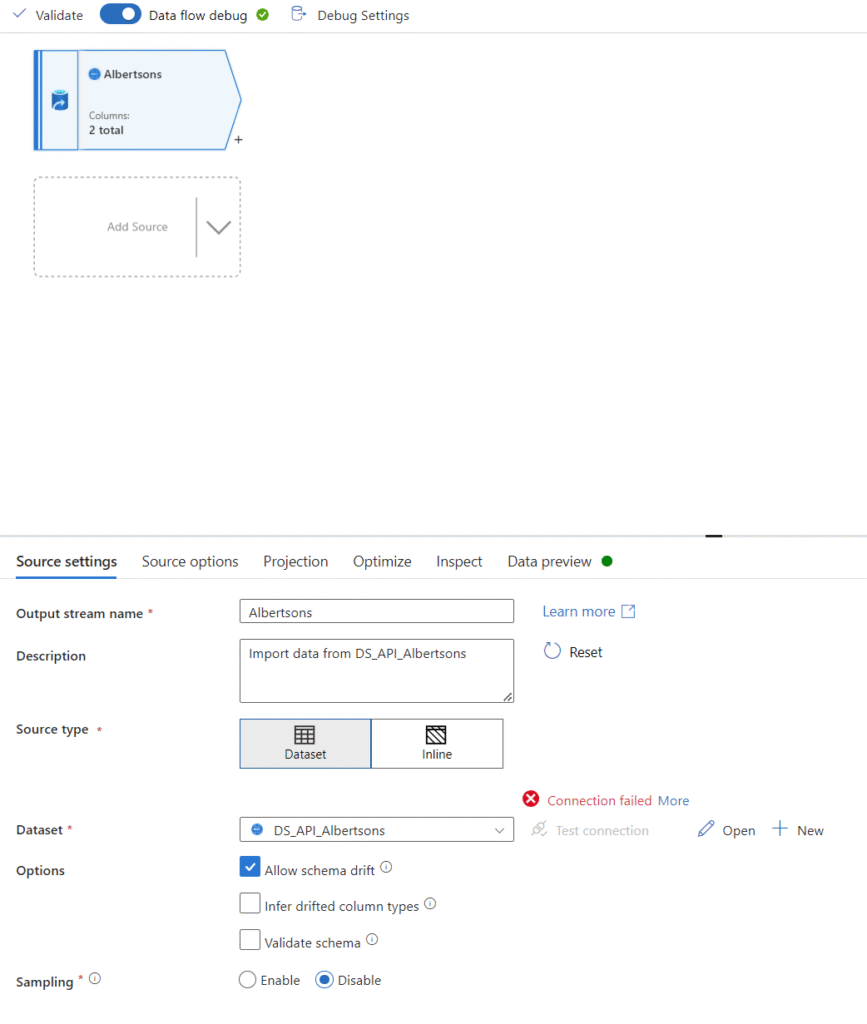
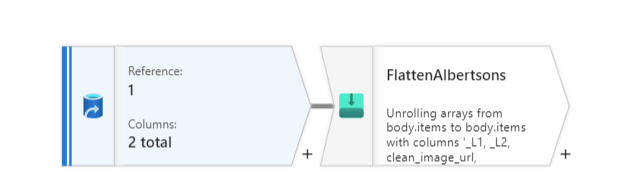
Our next step is to write the ETL itself within the dataflow section of ADF. Let’s start by creating a new dataflow and pulling in data from one of our datasets. You can see below that I’ve started with Albertsons. We just need to set the dataset field to our Albertsons dataset and leave all the other settings default. In Azure Data Factory, you’ll need to start a debug session (use this sparingly as it incurs nominal charges) in order to work with live data and test configurations, so at the top, you can enable data flow debug mode. Note that if you try to test the connection in the source settings window, you will get an error. This is because it’s trying to test only the base URL from the linked service which returns an error 404 as the API is expecting parameters. On the last tab, refreshing the data preview will let you drill into the actual API results (although it’s not too intuitive as the results are in the form of nested JSON).

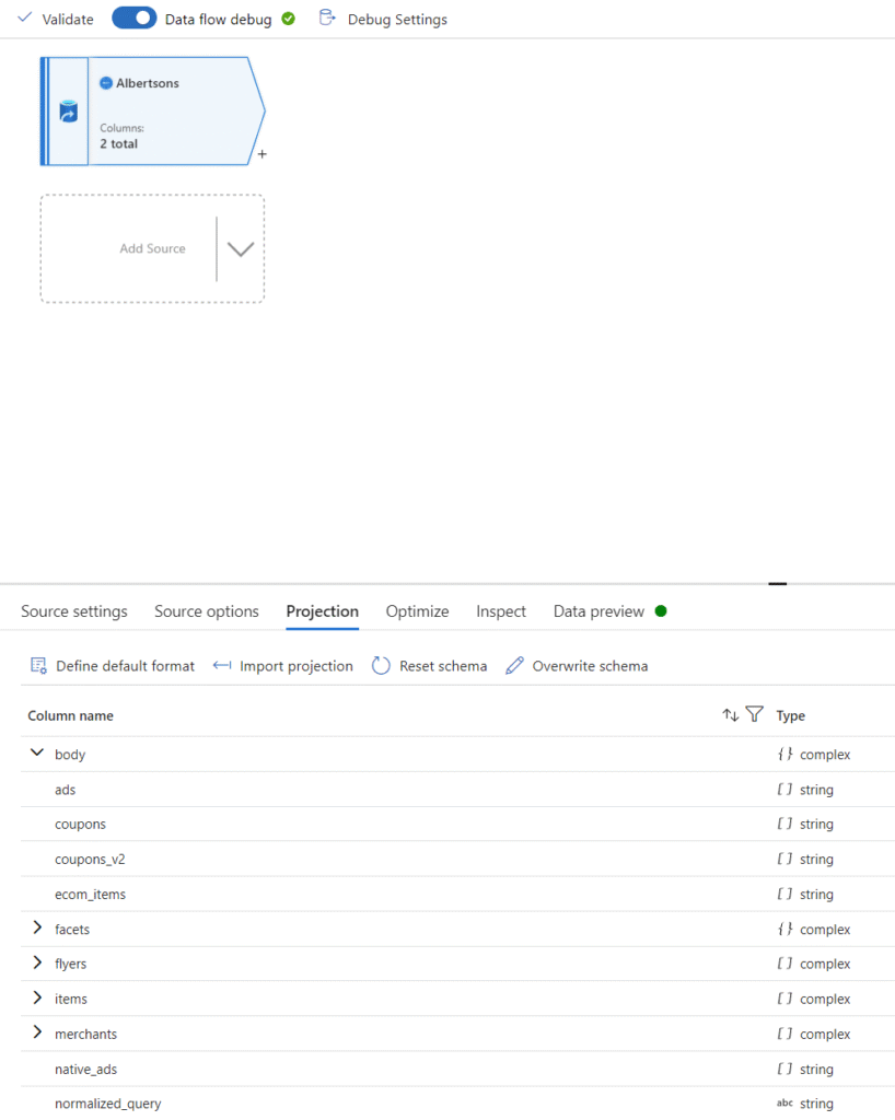
To proceed, we need to understand the structure of the returned data from the API. Let’s look at the schema of the data. This can be done in the Projections tab. Once debug mode is enabled, click ‘import projection’ to have ADF import the schema from the API. With this, you can drop down the ‘body’ column and see the nested structure within.

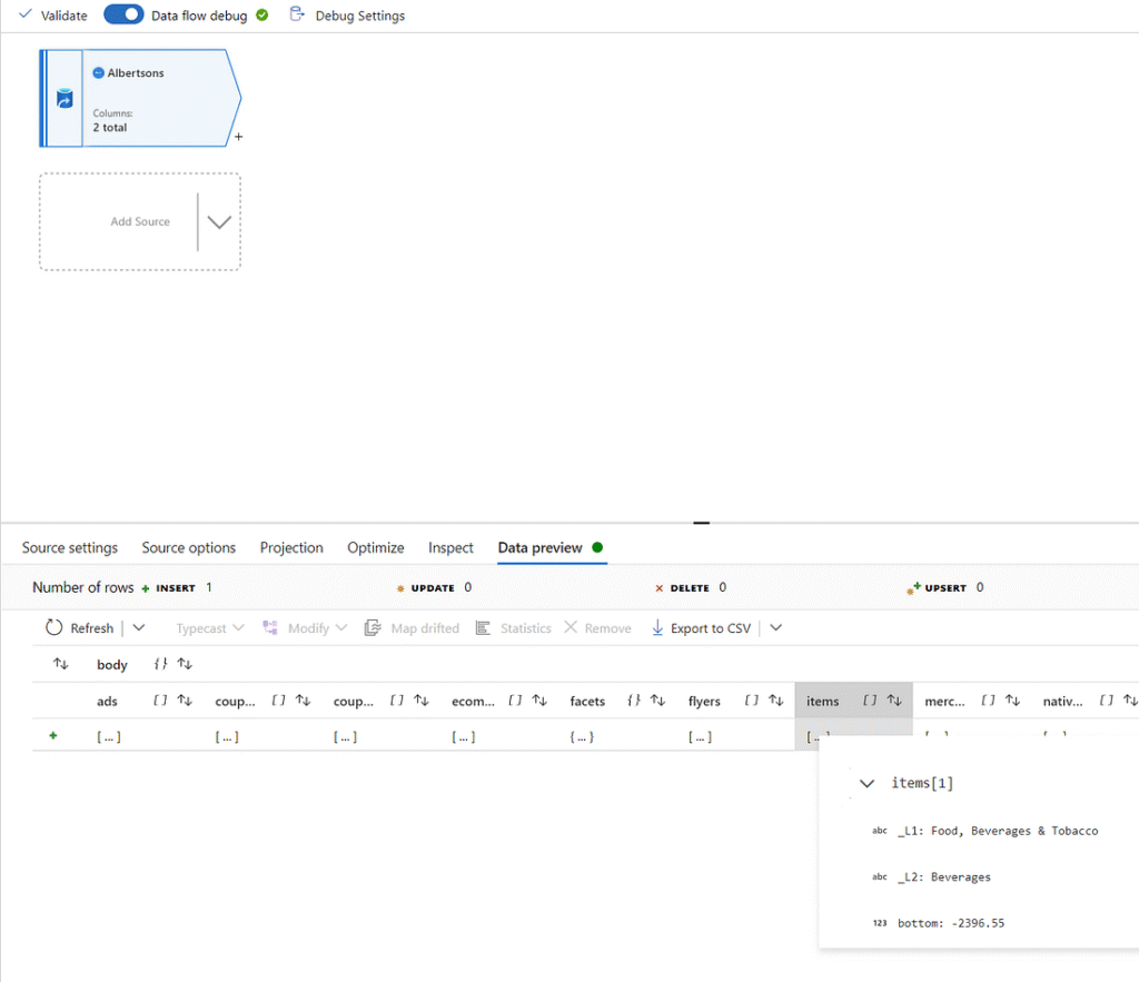
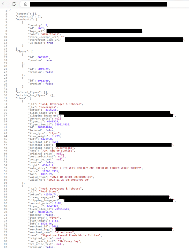
The data we want to pull is stored in the ‘items’ column within ‘body’. We can determine this by looking at the actual data returned by the API. There are two easy methods we can use to do this. One is to look at the data preview tab and click the […] under ‘items’, which can further be expanded to view individual items as dropdowns. You can also grab the actual API URL for Albertsons and paste it into Microsoft Edge (Chrome will not format the JSON in a friendly format at the time of writing this blog).

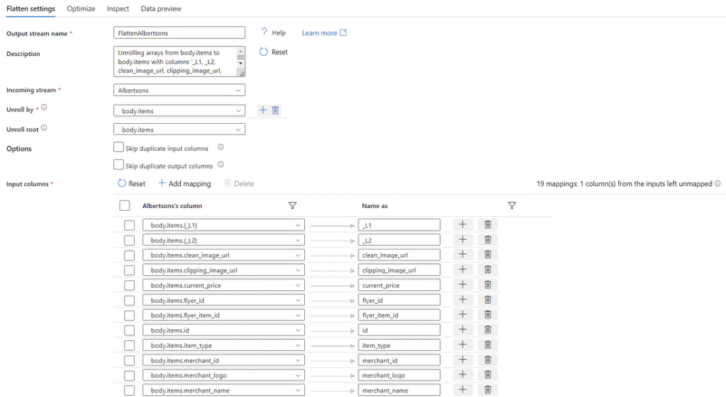
Since we have determined that the results are in the shape of nested JSON, we will need to flatten the data before manipulating it. Click the little ‘+’ to the bottom right of the source object in the GUI and add a ‘Flatten’ transformation. The setting ‘Unroll by’ tells ADF which attribute we want to unroll, and the setting ‘Unroll root’ tells ADF the root of the data to unroll. We will set both to ‘body.items’ as we want to see the contents within ‘items’ and we don’t care about attributes outside of ‘items’.

Below these settings we can reset the column mappings to see what columns we will bring in, and what they will be named. Let’s take this opportunity to filter out some of the attributes we don’t want. Remove the mapping for ‘bottom’, ‘indexed’, ‘item weight’, ‘left’, ‘premium’, ‘right’, ‘score’, and ‘top’ by clicking the garbage bin icon next to those attributes.

The next step in this process is to union all the datasets together, so let’s duplicate these two activities for the remaining four sources. Unfortunately, I am not aware of a way to clone these, they will need to be created manually (including the debug session to import projection for the flatten activity to see the schema).

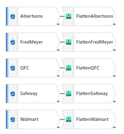
Let’s union these datasets together so we can work with the data as a whole. To do this, click the plus and select the ‘Union’ transformation. Within the settings you can select the incoming stream and the union streams. To make the UI diagram look the best, I suggest the incoming stream is set to the transformation that is on the top row of your diagram.

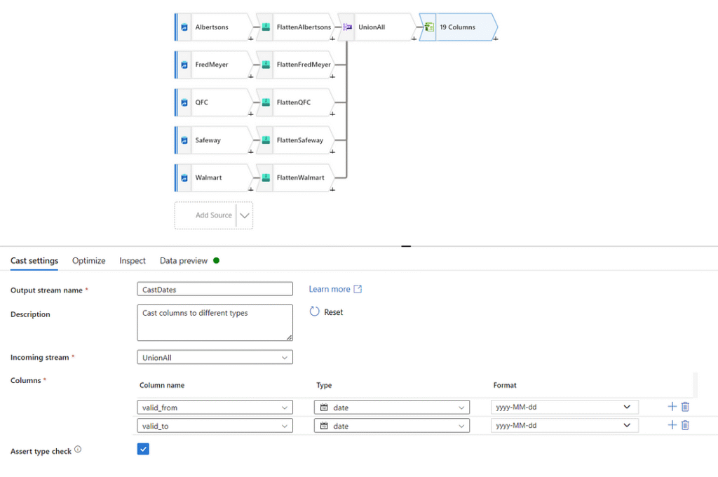
Now that the data is all together, there are a few cleaning tasks to complete before we send this data to our SQL DB. It doesn’t really matter which order these are performed in, but we need to cast the dates from strings to dates, add a couple of columns of our own, and filter out inactive advertisements.

The date attributes that come in from this API are initially identified as strings by Azure Data Factory, and they include date and time together in one attribute. We can see this by previewing the data in ADF.

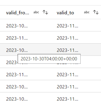
The only two date attributes we have are the ‘valid_to’ and ‘valid_from’ attributes telling us the start and end date of an advertisement. For our purposes, we only care about the date portion of this, so we can cast these attributes to be handled as dates. To do this, let’s create a new transformation of type ‘Cast’, and tell ADF that these attributes should be treated as dates. We can also specify the exact format we want them in. Let’s keep the date format the same as it was in v1 and v2: yyyy-MM-dd.

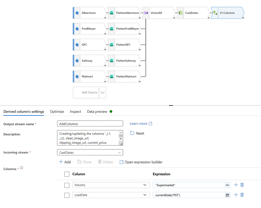
To be consistent with previous versions as well as knowing when we loaded data, let’s add two columns. To add columns, we can use the transformation ‘Derived Column’. The first attribute we will add is ‘Industry,’ which we will hardcode to “Supermarket”. The second attribute we will add is ‘LoadDate,’ which we will set to ‘currentDate(‘PST’)’. More information on the expression language used in Azure Data Factory can be found here: Expression functions in mapping data flow. Last year I originally capitalized the first letter of these added attributes, but in hindsight I should have kept them lowercase to remain consistent with the rest of the attributes.

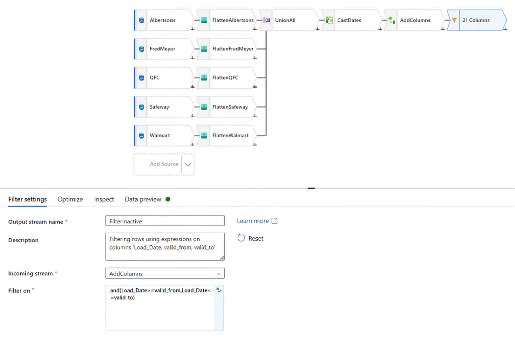
The final transformation we want to make is filtering out inactive advertisements. Through testing this data over time, I found instances where the current date does not fall within the time window specified by ‘valid_from’ and ‘valid_to’ for certain advertisements. We’re only interested in capturing snapshots of active sales, therefore we will filter out any advertisement that is not active. To accomplish this, we will use a filter transformation with the following expression.

and(Load_Date>=valid_from,Load_Date<=valid_to)

This leaves us with the data in the right format to be ingested by the SQL stored procedure we wrote earlier. The final step in completing this dataflow is assigning it a sink. As we have already created the dataset pointing to our staging table, let’s add it as a final transformation. Create a transformation of type ‘Sink’ and point it to your SQL DB. You’ll also need to inform ADF to execute our stored procedure after loading, which is done in the ‘Settings’ tab as a post SQL script.

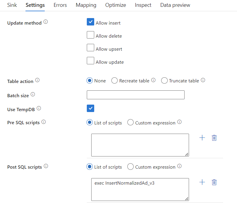
exec InsertNormalizedAd_v3

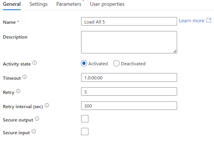
Remember to validate and publish your changes. Now that our datasets, linked services, and dataflow are set up, we need a way to trigger this to run. Let’s build a pipeline to encapsulate our dataflow, as triggers only function over pipelines. Create a new pipeline from the ‘Pipeline’ tab and drag and drop ‘data flow’ from the ‘Move and Transform’ header of activities. Configure this activity similar to how we configured the transformations.

Give the activity a name, select a maximum run time and number of retries. When I initially undertook this project, I did not expect the pipeline to fail as often as it did due to API timeout, so I did not set it to retry at all. I suggest setting it to retry five times with a five-minute break between attempts. Although losing data is not very detrimental as advertisements do not change on a daily basis, frequent data losses over multiple days in a row could risk losing some advertisements. More information on these failures and the impact can be seen in this follow-up post.

On the second tab, you will find the prompt asking which dataflow to run. Select your dataflow and leave the rest of the settings as default.

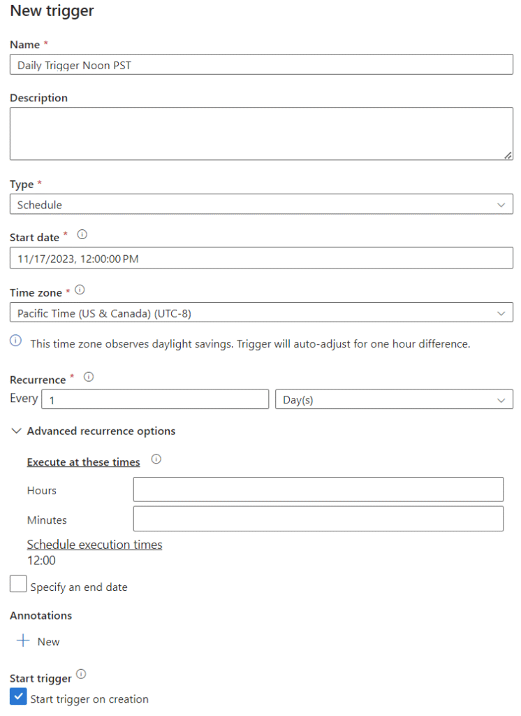
With the pipeline validated and published, the final step is to build a trigger. Within the pipeline GUI, you will see a button at the top called ‘Add Trigger.’ Click this and navigate to creating a new trigger. Set up the trigger for the frequency you desire. In this case, we want a daily run to occur at noon. We also want it to trigger once immediately when we create the trigger to test functionality.

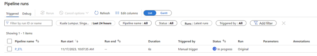
Once you trigger it to run, you can go to the ‘Monitor’ tab to watch the progress. Initially, it will show up as ‘In Progress,’ after which it will either fail or succeed. If it fails, you can rerun it from this view. In my case, it succeeded on the first attempt.

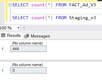
Seeing Results in SQL Server

It’s great to see a message of success in ADF, but seeing the data populated in SQL is much more reassuring. At this point, you can go back into SSMS or your preferred SQL platform and query your v3 tables. A simple count of rows in the fact table and the staging table (staging should be empty) will suffice to prove that it worked, but it’s also nice to see the data in a readable format.

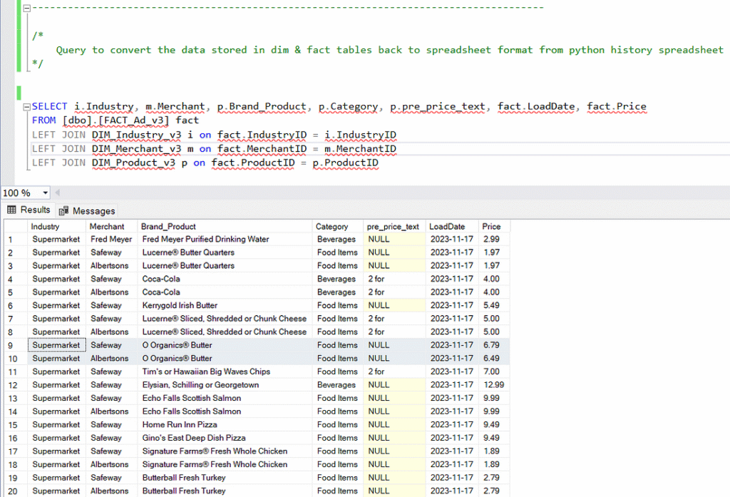
To see the data put back into a friendly format, use the following query.

SELECT 
    i.Industry,
    m.Merchant,
    p.Brand_Product,
    p.Category,
    p.pre_price_text,
    fact.LoadDate,
    fact.Price
FROM [dbo].[FACT_Ad_v3] fact
LEFT JOIN DIM_Industry_v3 i ON fact.IndustryID = i.IndustryID
LEFT JOIN DIM_Merchant_v3 m ON fact.MerchantID = m.MerchantID
LEFT JOIN DIM_Product_v3 p ON fact.ProductID = p.ProductID

You have now automated the process of pulling data from an API using ADF into a (kind of) normalized relational database! It’s easy to immediately start looking for interesting observations, such as if you are looking for O Organics Butter, you’ll find a better price at Albertsons than at Safeway.

Visualizing the Data

Since the underlying data did not change other than the addition of the ‘LoadDate’ attribute, the v3 report dashboard is an exact replica of the v2 report dashboard.

← Back to Home

Flyers 4 – Flyers v3: Azure Data Factory